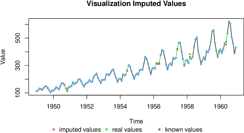
Handle Missing Values in Time Series Datasets: 10 Best Techniques
When working with time series datasets, encountering missing values is not uncommon. However, these missing values can significantly impact the accuracy and reliability of data analysis and predictions. Therefore, it becomes crucial to handle them appropriately. In this article, we will explore different techniques for handling missing values in time series datasets, along with examples, to ensure the integrity and quality of the data.

Table of Contents
Introduction
Time series datasets are widely used in data analysis and forecasting. However, missing values can pose a challenge in deriving accurate insights and predictions. Handling missing values effectively is essential to ensure the reliability of time series analysis. In this article, we will explore various techniques that can be employed to handle missing values in time series datasets.
Understanding Missing Values in Time Series Datasets
Before diving into the techniques, let’s understand the nature of missingness in time series datasets. Missing values can occur in the following ways:
- Missing Completely at Random (MCAR): The missingness is random and unrelated to any variables or patterns in the data.
- Missing at Random (MAR): The probability of a value being missing depends on other observed variables within the dataset.
- Missing Not at Random (MNAR): The missingness is related to the missing values themselves and not influenced by other observed variables.
Now, let’s explore the techniques for handling missing values in time series datasets.
Technique 1: Listwise Deletion
Listwise deletion, also known as complete case analysis, involves removing rows with missing values from the dataset. This technique is simple to implement but can result in a significant loss of data. Listwise deletion is suitable when the missingness is completely random and does not introduce bias.
Example:
Suppose we have a time series dataset with daily temperature recordings. Using listwise deletion, if there are missing values for certain days, we remove those entire rows from the dataset.
Technique 2: Forward Filling
Forward filling, also called last observation carried forward (LOCF), replaces missing values with the last observed value. This technique assumes that the missing values have the same value as the preceding observation.
Example:
Consider a monthly sales dataset where some months have missing values. Using forward filling, we replace the missing values with the sales value from the previous observed month.
Technique 3: Backward Filling
Backward filling, also known as next observation carried backward (NOCB), replaces missing values with the next observed value. It assumes that the missing values have the same value as the subsequent observation.
Example:
Suppose we have a daily stock price dataset where some days have missing values. Applying backward filling, we replace the missing values with the stock price from the following observed day.
Technique 4: Linear Interpolation
Linear interpolation estimates missing values by computing the average between the previous and next observed values. It assumes a linear relationship between adjacent observations.
Example:
Consider a time series dataset representing the hourly electricity consumption. If there are missing values, linear interpolation estimates them by taking the average of the preceding and succeeding observed values.
Technique 5: Seasonal Decomposition of Time Series
Seasonal decomposition of time series (STL) decomposes a time series into trend, seasonal, and residual components. By identifying patterns in each component, missing values can be estimated.
Example:
Suppose we have a quarterly revenue dataset. Using seasonal decomposition, we decompose the series into trend, seasonal, and residual components. Based on the identified patterns, we estimate the missing values in each component.
Technique 6: Time Series Imputation
Time series imputation techniques estimate missing values based on the statistical properties of the time series. Common methods include mean imputation, median imputation, or regression imputation.
Example:
Consider a daily stock market dataset with missing closing prices. Using time series imputation, we can estimate the missing values by calculating the mean or median of the observed closing prices.
Technique 7: K-nearest Neighbors Imputation
K-nearest neighbors imputation estimates missing values by identifying the K-nearest neighbors based on available features. The missing values are then filled with the average of their values.
Example:
Suppose we have a monthly weather dataset with missing humidity values. Using K-nearest neighbors imputation, we identify the K-most similar months based on other weather variables and fill the missing humidity values with their average.
Technique 8: Moving Average Imputation
Moving average imputation replaces missing values with the average of the previous and next observations. The size of the moving window determines the smoothness of the imputed values.
Example:
Consider a weekly website traffic dataset with missing values. Applying moving average imputation, we replace the missing values with the average of the previous and subsequent observed traffic.
Technique 9: Multiple Imputation
Multiple imputation generates multiple plausible values for missing observations based on a model that considers the relationships between variables. It accounts for the uncertainty associated with missing values.
Example:
Suppose we have a monthly sales dataset with missing values. Using multiple imputation, we create multiple sets of plausible values for the missing sales based on a model that considers other relevant variables.
Technique 10: Feature Engineering Techniques
Feature engineering techniques involve creating additional features that capture information related to missing values. For example, adding a binary indicator variable that denotes whether a value is missing can help capture the missingness pattern.
Example:
In a customer churn prediction dataset, we can create a binary feature indicating whether a customer’s demographic information is missing. This additional feature provides valuable information for predicting churn.
Handling Missing Values in Machine Learning Models
When using time series datasets in machine learning models, handling missing values is crucial. Some common approaches include:
- Model-based Imputation: Use machine learning models to predict missing values based on observed data. Techniques such as regression, random forests, or deep learning can be employed for this purpose.
- Time Series Cross-Validation: Implement time series cross-validation techniques to assess the model’s performance while considering the temporal nature of the data and the presence of missing values.
- Feature Selection: Select relevant features while considering the presence of missing values. Discard features with excessive missingness or utilize feature engineering techniques to improve model performance.
Conclusion
Handling missing values in time series datasets is essential for accurate analysis and prediction. By employing appropriate techniques such as listwise deletion, forward filling, backward filling, linear interpolation, time series imputation, or utilizing machine
learning models, we can ensure the integrity and quality of the data. The choice of technique depends on the nature of missingness and the specific characteristics of the time series dataset.
FAQs
- Q: What are the common reasons for missing values in time series datasets?
A: Missing values in time series datasets can occur due to various reasons such as sensor failures, data corruption, or unavailability of data during certain time periods. - Q: How can missing values impact time series analysis and predictions?
A: Missing values can lead to gaps in the dataset, making it challenging to derive meaningful insights and accurate predictions. The presence of missing values can introduce bias and affect the statistical properties of the data. - Q: Are there any drawbacks to listwise deletion?
A: Listwise deletion can result in a significant loss of data, especially when missingness is not completely random. It may also introduce bias if the missingness pattern is related to the outcome variable. - Q: What is the purpose of seasonal decomposition of time series?
A: Seasonal decomposition of time series aims to identify the trend, seasonal, and residual components within a time series. By decomposing the series, missing values can be estimated based on the identified patterns in each component. - Q: How can feature engineering help in handling missing values?
A: Feature engineering techniques, such as creating additional features that capture missingness patterns, can provide valuable information for predictive models. Adding binary indicators or imputation flags can improve the model’s performance in handling missing values.


